Lab #1: The Buggy Lab
Partners: Aayush Chopra and Andy Chen
How does time affect the final position of the buggy?
Independent Variable: seconds. Dependent Variable: position in cm
Controls: The controls of this experiment are the buggy, the initial position, and the floor. In order to ensure that these are all kept the same, we started each experiment in the same exact starting point using the same buggy. In all trials the buggy was at a complete stop before being turned on and was driven in the same direction over the same terrain each time.
Collection of Data: To collect accurate data we used a meter stick and a stopwatch. The stopwatch was used to time the trail to certify the buggy is traveling for the correct amount of time. Then when stopped, we used the meter stick to measure the final position from the initial starting position.
Procedure
We measured how far the buggy could travel in a certain period of time.
Materials
Meter Stick, Garmin Watch, Buggy
(diagram below)
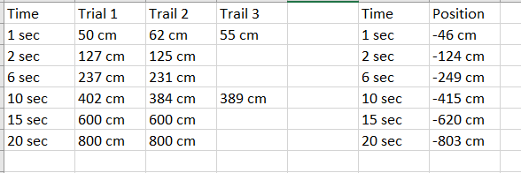
Raw Data
(pictured below the materials)
Processed Raw Data
The different trials for each data point were averaged out.
The graphs are depicted below the Raw Data
How does time affect the final position of the buggy?
Independent Variable: seconds. Dependent Variable: position in cm
Controls: The controls of this experiment are the buggy, the initial position, and the floor. In order to ensure that these are all kept the same, we started each experiment in the same exact starting point using the same buggy. In all trials the buggy was at a complete stop before being turned on and was driven in the same direction over the same terrain each time.
Collection of Data: To collect accurate data we used a meter stick and a stopwatch. The stopwatch was used to time the trail to certify the buggy is traveling for the correct amount of time. Then when stopped, we used the meter stick to measure the final position from the initial starting position.
Procedure
We measured how far the buggy could travel in a certain period of time.
- We placed the buggy down on the ground in the initial position.
- Then turned on the stopwatch as soon as we turned on the buggy’s engine.
- When the time hit the amount of the seconds we were measuring that trial we stopped the buggy.
- Then using the meter stick we measured out the distance between the buggy and the starting position.
- We collected a total of 6 data points and for each data point we did 2-3 trails.
Materials
Meter Stick, Garmin Watch, Buggy
(diagram below)
Raw Data
(pictured below the materials)
Processed Raw Data
The different trials for each data point were averaged out.
The graphs are depicted below the Raw Data

Interpretation of Data
Conclusion
The main conclusion able to be drawn from this expirament is that as time increases, the position of the buggy's position will move father away at an almost linear rate.
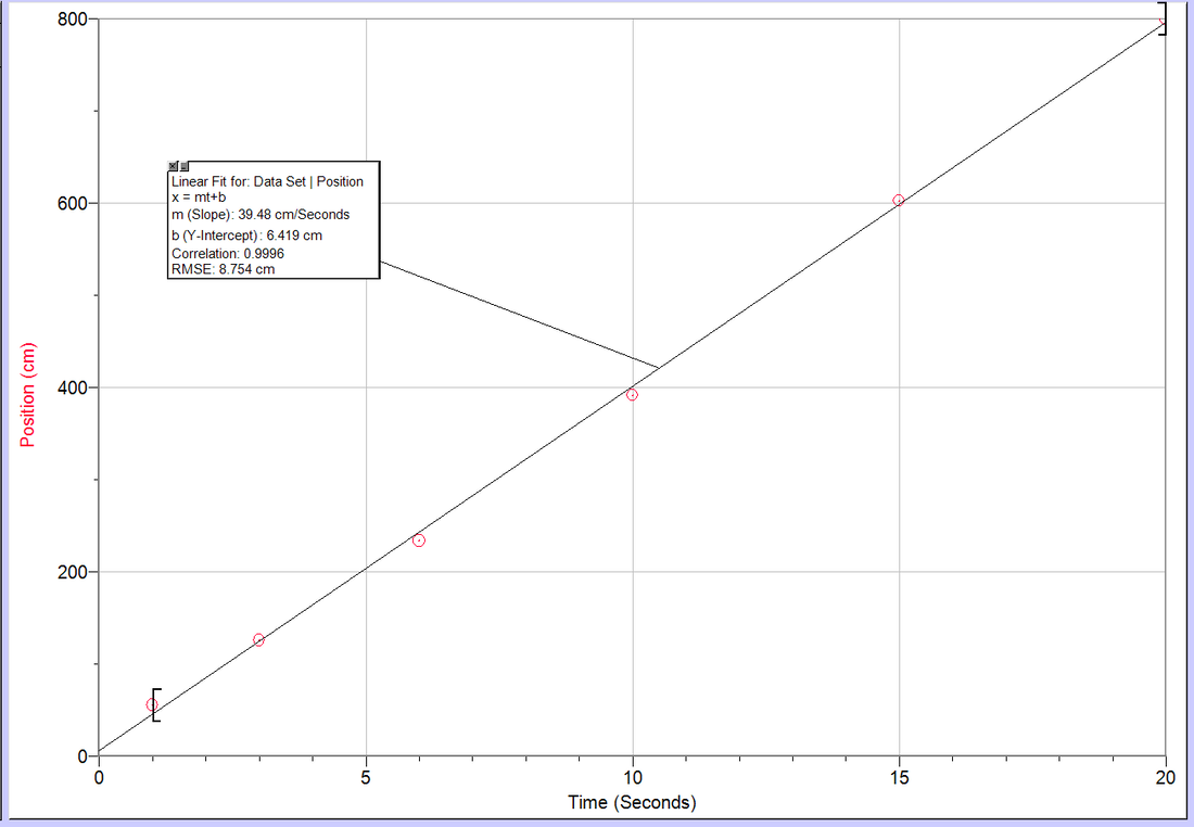
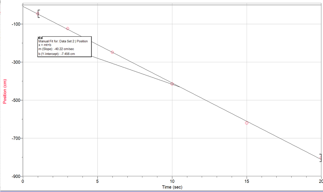
The second conclusion that can be drawn from this data and expirament is how the relationship between position and time represents the velocity of the function.Using the collected data displayed in the graphs (Fig. 3, Fig. 4) a line of best fit was fit to both of these separate data points. Both of these data plots were then fit to a linear model. The steady speed of the cart made it so that the linear model made the most sense concerning a fit. Fitting the data points gave both the experiments an equation for the data:
Position= 39.48(elapsed time) + 6.419 Position= -40.22(elapsed time) - 7.456
From this equation we can come to the conclusion of an expression for velocity and the derived equation for it. Each value in the respective equations can be assigned a variable. The Y value of the equation, Position (x), can now be expressed as Final Position (xf). SImilarly the y intercept can be expressed as Initial Position (xi) as it is the starting point of the buggy where time is zero. Because velocity is an expression for speed and direction, it is modeled by the slope, which is sign and magnitude. From this we can arrive at the new equation
xf= v(elapsed time) + xi
Which can be turned into
v= (xf - xi)/elapsed time
This conclusion proves that the buggy is moving at a near constant velocity in each of the experiments and using this graph an equation to determine the velocity of a moving object.
Evaluating and Improving Procedures
- Slope: The slopes of the graphs indicate the direction and the speed. The steeper the slope, the faster the buggy is moving. In the first experiment the buggy is moving 39.48 cm in one second and 40.22 cm in one second in Experiment 2. The negative or positive sign in front of the slope indicates in what direction the buggy is moving. Experiment 2 has a negative slope so it is moving in the negative direction from the initial position. The combination of direction and speed is velocity, so the slope of these graphs indicate the velocity of the buggy. The new derived equation of velocity is expressed as v= (final position- initial position)/elapsed time.
- Y intercept: The Y intercept is the position of the buggy when time equals zero. The Y intercept of the first graph is 6.419 and -7.456 for the second graph.
- Confidence: We are confident in the range of data. It is a large range, varying from 1 second all the way to 20 seconds. However, there is a lack of confidence in the number of data points because we only collected 6 for each of the two experiments. Also, there is a lack of confidence in the number of trials in the second experiment. There is only one trail for each data point lending to some lack of confidence.
Conclusion
The main conclusion able to be drawn from this expirament is that as time increases, the position of the buggy's position will move father away at an almost linear rate.
The second conclusion that can be drawn from this data and expirament is how the relationship between position and time represents the velocity of the function.Using the collected data displayed in the graphs (Fig. 3, Fig. 4) a line of best fit was fit to both of these separate data points. Both of these data plots were then fit to a linear model. The steady speed of the cart made it so that the linear model made the most sense concerning a fit. Fitting the data points gave both the experiments an equation for the data:
Position= 39.48(elapsed time) + 6.419 Position= -40.22(elapsed time) - 7.456
From this equation we can come to the conclusion of an expression for velocity and the derived equation for it. Each value in the respective equations can be assigned a variable. The Y value of the equation, Position (x), can now be expressed as Final Position (xf). SImilarly the y intercept can be expressed as Initial Position (xi) as it is the starting point of the buggy where time is zero. Because velocity is an expression for speed and direction, it is modeled by the slope, which is sign and magnitude. From this we can arrive at the new equation
xf= v(elapsed time) + xi
Which can be turned into
v= (xf - xi)/elapsed time
This conclusion proves that the buggy is moving at a near constant velocity in each of the experiments and using this graph an equation to determine the velocity of a moving object.
Evaluating and Improving Procedures
- More Data points within 1 to 20 seconds
- Better way to stop the cart at the end of time
- Find a better way to time the cart instead of starting and stopping a stopwatch
- Have more trails for each data point to maximaze accuracy
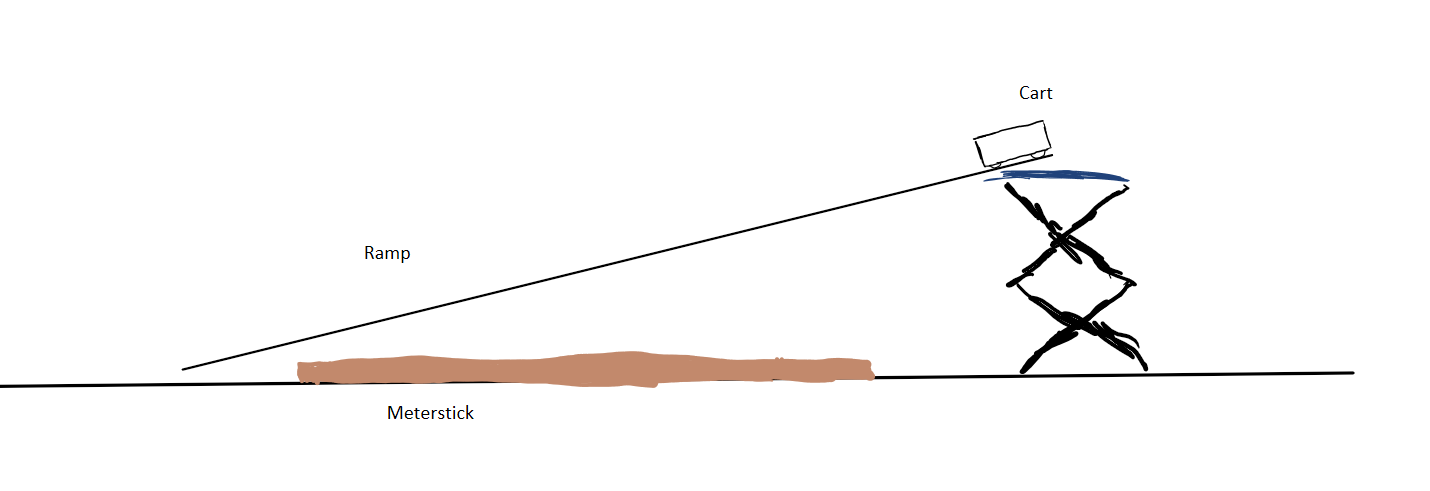
Lab #2 Cart on Ramp 9-30
Partners: Matt Singer and Aayush Chopra
How does time affect the position of the cart when rolling down a ramp?
Independent Variable: time Dependent Variable: position
The controls of the experiment are the cart, same ramp, same starting position on the ramp, and the angle of the ramp. To ensure the control of these controlled variables we used the same cart, and the same ramp. The ramp was not tampered with so the height stayed the same. Also only one trail was performed because all data points were selected from the trail so the constants among other trails are not a part of this experiment. The constants stay the same within the trial however.
For the collection of data we took a video of the cart rolling down the ramp. Putting this video into Logger Pro, we scaled this video so that the time of the experiment started when the cart was first released. We also used a meterstick to match the number of pixels from the computer for a single meter so we could accurately measure the position. Then by playing the video frame by frame, we were able to plot these points directly into a graph.
We measured the position of the cart in respect to time when rolling down a ramp
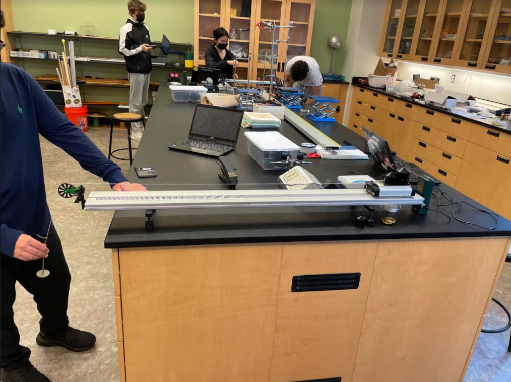
- We set up our camera to video the cart and placed a meter stick in front of the ramp
- We placed the cart at the top of the ramp at a complete stop and held it. We then released the cart and caught it as it fell off the ramp.
- We imported the video into Logger Pro and Set the scale for a meter and the frame in the video when the cart begins to move.
- Frame by frame we marked the position of the cart and it plotted into the graph.
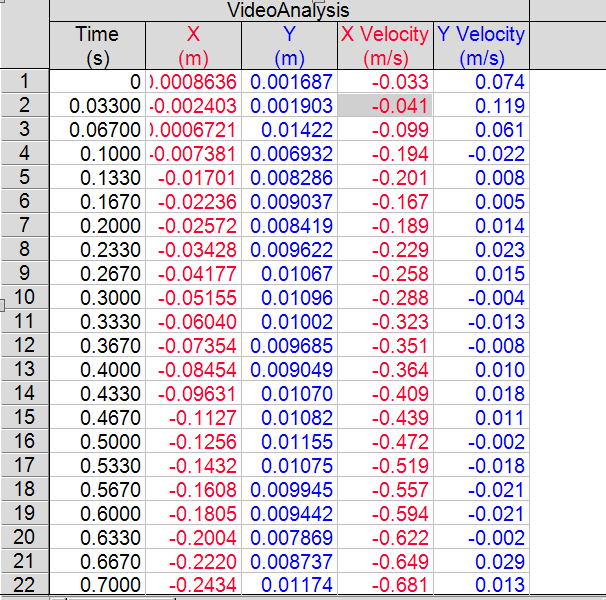
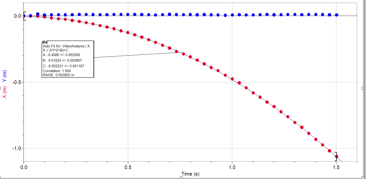
The Position vs. Time graph(Fig 3) has an equation of x=-0.458t^2 -0.0183t -0.00323.
This equation is significant because it fits a quadratic model rather than a linear model. The slope is getting sleeper as time moves on. The sign of the slope is negative meaning that the cart is getting farther and farther away from the initial position in a negative direction.
The y intercept of the graph is 0.00086 which is practically zero. After Zero seconds the cart has not moved at all from the initial position of the origin.
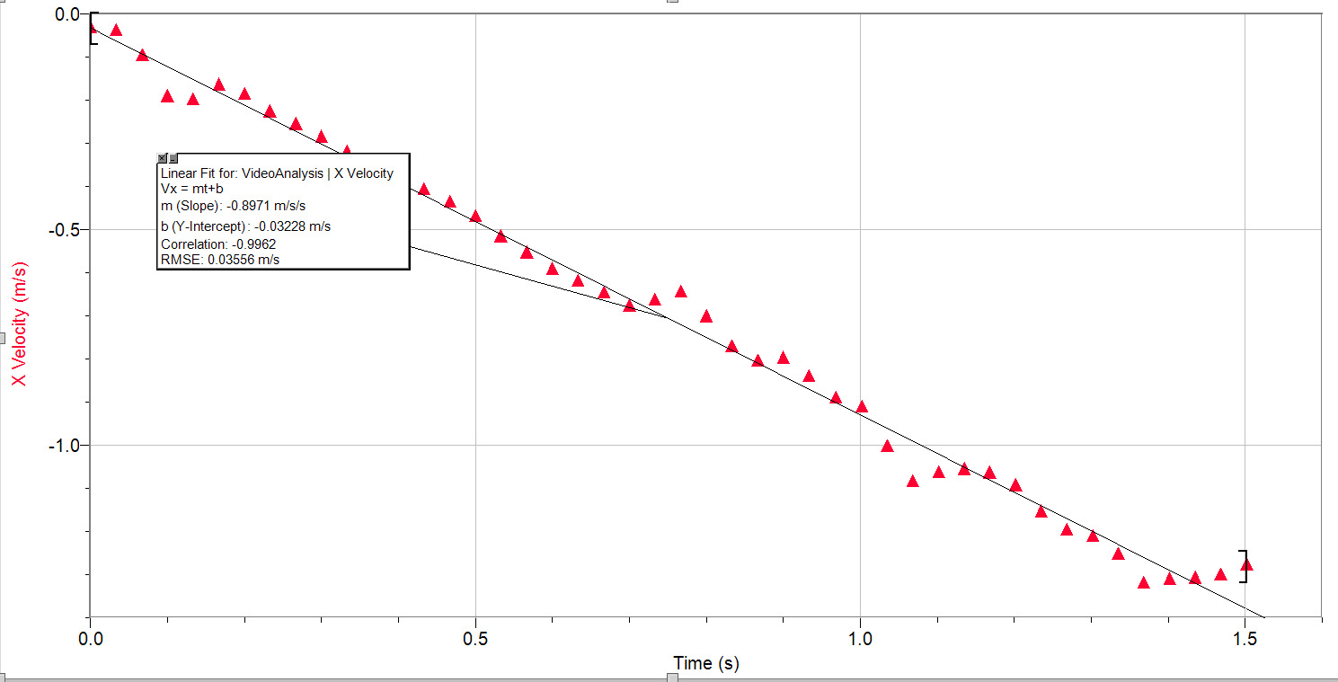
For the Velocity Time Graph(Fig 4) taken from the position time graph, the equation is V=-0.8971t -0.0323
The slope means that the velocity time graph is at a constant deceleration and the Velocity is decreasing as the time moves on. Although the Velocity is becoming negative, the object is becoming faster and picking up speed. This can be expressed through a term called Acceleration. Acceleration is defined as the change in velocity over time, and is the slope of the Velocity Time graph. This definition lets us determine the equation for a (acceleration). Therefore, the equation for acceleration is a=change in velocity/change in time.
The Y intercept of this graph is -0.032 which means the velocity is approximately zero. This entails that the cart has not started moving yet at the point when t=0.
Conclusion
The Purpose of this lab is to analyze the relationship between position and time and how velocity and acceleration affect this relationship. After this experiment, we were able to conclude that when placed on a ramp and traveling in a negative direction, the slope and velocity got steeper in a negative direction. We observed that in both of our graphs. Our first graph displayed that by fitting a quadratic function and having a negative slope. The second graph portrayed the negative change in velocity as the graph had a negative slope. These overall conclusions led us to discover acceleration and its expression and relationship with velocity. We concluded it is the slope of a velocity time graph and represents the change in velocity. This lab was very important in now understanding linear and quadratic relationships between position and time and how it is impacted by velocity and acceleration.
Improving and Evaluating.
We are very confident in our experiment. Because all the data was collected by a computer, only one trial per each data point was needed. Also there are a lot of data points so that is a reason for confidence. One lack of confidence could come from too small a range of data even though the range was pretty large. The range in data points is definitely the area with the least amount of confidence. One improvement this lab could make is to make the track longer to collect a larger range of data.
This equation is significant because it fits a quadratic model rather than a linear model. The slope is getting sleeper as time moves on. The sign of the slope is negative meaning that the cart is getting farther and farther away from the initial position in a negative direction.
The y intercept of the graph is 0.00086 which is practically zero. After Zero seconds the cart has not moved at all from the initial position of the origin.
For the Velocity Time Graph(Fig 4) taken from the position time graph, the equation is V=-0.8971t -0.0323
The slope means that the velocity time graph is at a constant deceleration and the Velocity is decreasing as the time moves on. Although the Velocity is becoming negative, the object is becoming faster and picking up speed. This can be expressed through a term called Acceleration. Acceleration is defined as the change in velocity over time, and is the slope of the Velocity Time graph. This definition lets us determine the equation for a (acceleration). Therefore, the equation for acceleration is a=change in velocity/change in time.
The Y intercept of this graph is -0.032 which means the velocity is approximately zero. This entails that the cart has not started moving yet at the point when t=0.
Conclusion
The Purpose of this lab is to analyze the relationship between position and time and how velocity and acceleration affect this relationship. After this experiment, we were able to conclude that when placed on a ramp and traveling in a negative direction, the slope and velocity got steeper in a negative direction. We observed that in both of our graphs. Our first graph displayed that by fitting a quadratic function and having a negative slope. The second graph portrayed the negative change in velocity as the graph had a negative slope. These overall conclusions led us to discover acceleration and its expression and relationship with velocity. We concluded it is the slope of a velocity time graph and represents the change in velocity. This lab was very important in now understanding linear and quadratic relationships between position and time and how it is impacted by velocity and acceleration.
Improving and Evaluating.
We are very confident in our experiment. Because all the data was collected by a computer, only one trial per each data point was needed. Also there are a lot of data points so that is a reason for confidence. One lack of confidence could come from too small a range of data even though the range was pretty large. The range in data points is definitely the area with the least amount of confidence. One improvement this lab could make is to make the track longer to collect a larger range of data.
Lab #3 Unbalenced Forces Lab
Partners: Jack Hughes, Tyler Fromovich
Experiment 1
Independent Value - Net Force in Newtons
Dependent Variable - Acceleration in m/s^2
Constants: Constants for this Lab are the same hangar, cart, pulley and string that makes up the system. The main Constant variable in this experiment however, is the Total Mass of the system (Kg). This is controlled by using the same number of the same weights for each data point. When increasing the force, weights are pulled off the cart and placed onto the hangar. This way the same total mass is still in the system.
Method For Collecting Data:
The Measurement of data was done using a motion detector that sent soundwaves out and collected them to determine the position of an object. This data was directly fed in Logger Pro and graphed on a Velocity Time graph. By selecting the portion of the graph with a steady increasing slope we were able to identify the acceleration, which is the slope.
Procedure:
Upon determining the amount of Force and weight we were going to use, we moved that amount of weight in little metal plates from the car to on top of the hangar. The hangar, connected by a thin string to the front of the cart which is positioned at the end of a 1 meter track, is draped over a pulley wheel. When the desired amount of mass is placed on the hangar we hold the hangar off the edge of the table. Then we turned on the motion sensor and let the hangar drop which in turn pulled the cart forward. Right before the hangar hit the ground we stopped the motion of the cart. Then looking at the slope of the Velocity Time graph, we then jotted down the acceleration for that specific force.
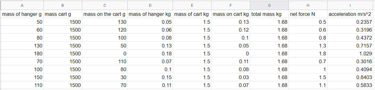
(Below Pictured is the materials and set up for the lab, Raw data, and processed data for experiment 1)
Experiment 1
Independent Value - Net Force in Newtons
Dependent Variable - Acceleration in m/s^2
Constants: Constants for this Lab are the same hangar, cart, pulley and string that makes up the system. The main Constant variable in this experiment however, is the Total Mass of the system (Kg). This is controlled by using the same number of the same weights for each data point. When increasing the force, weights are pulled off the cart and placed onto the hangar. This way the same total mass is still in the system.
Method For Collecting Data:
The Measurement of data was done using a motion detector that sent soundwaves out and collected them to determine the position of an object. This data was directly fed in Logger Pro and graphed on a Velocity Time graph. By selecting the portion of the graph with a steady increasing slope we were able to identify the acceleration, which is the slope.
Procedure:
Upon determining the amount of Force and weight we were going to use, we moved that amount of weight in little metal plates from the car to on top of the hangar. The hangar, connected by a thin string to the front of the cart which is positioned at the end of a 1 meter track, is draped over a pulley wheel. When the desired amount of mass is placed on the hangar we hold the hangar off the edge of the table. Then we turned on the motion sensor and let the hangar drop which in turn pulled the cart forward. Right before the hangar hit the ground we stopped the motion of the cart. Then looking at the slope of the Velocity Time graph, we then jotted down the acceleration for that specific force.
(Below Pictured is the materials and set up for the lab, Raw data, and processed data for experiment 1)
Experiment 2
Independent Variable: Total Mass
Dependent Variable: Acceleration
Constants: Constants for this Lab are the same hangar, cart, pulley and string that makes up the system. The constant variable of this lab though is the Net Force. The Net Force is represented as the amount of weight on the hangar. By keeping the force constant, the total mass of the system is the only thing that will be changing the acceleration.
Method For Collecting Data: The Measurement of data was done using a motion detector that sent soundwaves out and collected them to determine the position of an object. This data was directly fed in Logger Pro and graphed on a Velocity Time graph. By selecting the portion of the graph with a steady increasing slope we were able to identify the acceleration, which is the slope.
Procedure: Upon determining the amount of total weight for that trial, we moved that amount of weight to the top of the car. We put no weight on the hangar in order to keep the Force constant. From this moment on, the experiment and the moving of the car is identical to the first experiment along with the data collection.
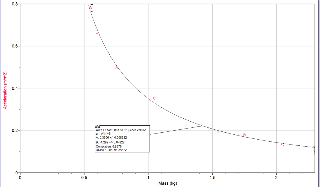
Below are the Raw and Processed Data for this Lab
Independent Variable: Total Mass
Dependent Variable: Acceleration
Constants: Constants for this Lab are the same hangar, cart, pulley and string that makes up the system. The constant variable of this lab though is the Net Force. The Net Force is represented as the amount of weight on the hangar. By keeping the force constant, the total mass of the system is the only thing that will be changing the acceleration.
Method For Collecting Data: The Measurement of data was done using a motion detector that sent soundwaves out and collected them to determine the position of an object. This data was directly fed in Logger Pro and graphed on a Velocity Time graph. By selecting the portion of the graph with a steady increasing slope we were able to identify the acceleration, which is the slope.
Procedure: Upon determining the amount of total weight for that trial, we moved that amount of weight to the top of the car. We put no weight on the hangar in order to keep the Force constant. From this moment on, the experiment and the moving of the car is identical to the first experiment along with the data collection.
Below are the Raw and Processed Data for this Lab
Conclusions
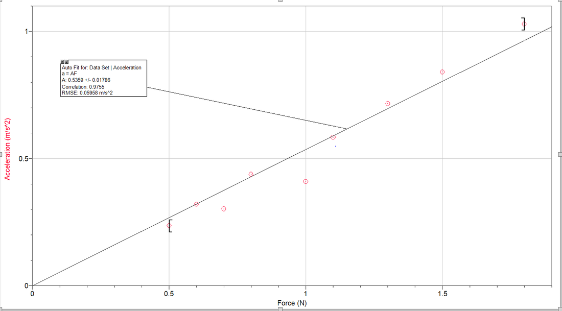
In conclusion, when looking at the data for both experiments, we were able to draw some main points about the relationship between the total mass of the system, the Force downward by the hangar, and the acceleration forward by the cart. For the first experiment, we observed a positive roughly linear relationship between the Force and the Acceleration. As we increased the Force of the hangar dropping, the acceleration would increase as well. The model and our data predicts the future data points and fit it to a trendline of the equation
a = 0.5359 F
This generally says that for every 1N increase exerted by the hangar, that the acceleration will increase by about 0.5359 m/s^2.
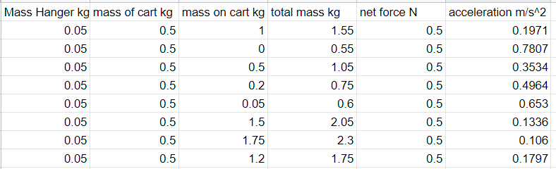
For the second experiment, we observe a negative relationship between Mass and Acceleration unlike the first experiment. As the mass of the object being moved decreases, the acceleration increases exponentially until the mass is zero. This means that as we add weight and mass increases, the acceleration will decrease very quickly and become much smaller until the hangar cannot move the cart. This graph is fit to a negative power function, with the equation being
a = 0.3506m^-1.292
When comparing the two relationships observed in these two experiments, the most important lies between Force, Acceleration, and Mass. From the two respective conclusions for each graph above, we can determine that as you increase the mass and keep the acceleration the same, the force must increase. We can also determine that if the acceleration is increased, but the mass stays the same, then the Force of the object must increase as well. From this we can conclude an equation for these three variables in the form of
F = ma
Evaluating and Improving
Some weaknesses and limitations were the weights being used in the lab and the number of trials. We were only mostly able to get 1 trail per data point with a couple of exceptions. This aids to some added uncertainty because of the possibility of a bad trail for that data point. Another possible issue in the lab was that the weights being used were increasing in large increments and often saw a large jump up in the amount from trail to trial. For example, within 1 to 2 kg, we were only able to get 3 data points in, and they were around 0.25 to 0.5 kg away from each other. As our weight increases, our data points seem to decrease which could possibly hurt the accuracy of our data at a higher mass. A way to possibly avoid and improve this problem would be to use weights that would more uniformly increase the mass to get an even and accurate spread of data.
In conclusion, when looking at the data for both experiments, we were able to draw some main points about the relationship between the total mass of the system, the Force downward by the hangar, and the acceleration forward by the cart. For the first experiment, we observed a positive roughly linear relationship between the Force and the Acceleration. As we increased the Force of the hangar dropping, the acceleration would increase as well. The model and our data predicts the future data points and fit it to a trendline of the equation
a = 0.5359 F
This generally says that for every 1N increase exerted by the hangar, that the acceleration will increase by about 0.5359 m/s^2.
For the second experiment, we observe a negative relationship between Mass and Acceleration unlike the first experiment. As the mass of the object being moved decreases, the acceleration increases exponentially until the mass is zero. This means that as we add weight and mass increases, the acceleration will decrease very quickly and become much smaller until the hangar cannot move the cart. This graph is fit to a negative power function, with the equation being
a = 0.3506m^-1.292
When comparing the two relationships observed in these two experiments, the most important lies between Force, Acceleration, and Mass. From the two respective conclusions for each graph above, we can determine that as you increase the mass and keep the acceleration the same, the force must increase. We can also determine that if the acceleration is increased, but the mass stays the same, then the Force of the object must increase as well. From this we can conclude an equation for these three variables in the form of
F = ma
Evaluating and Improving
Some weaknesses and limitations were the weights being used in the lab and the number of trials. We were only mostly able to get 1 trail per data point with a couple of exceptions. This aids to some added uncertainty because of the possibility of a bad trail for that data point. Another possible issue in the lab was that the weights being used were increasing in large increments and often saw a large jump up in the amount from trail to trial. For example, within 1 to 2 kg, we were only able to get 3 data points in, and they were around 0.25 to 0.5 kg away from each other. As our weight increases, our data points seem to decrease which could possibly hurt the accuracy of our data at a higher mass. A way to possibly avoid and improve this problem would be to use weights that would more uniformly increase the mass to get an even and accurate spread of data.
Unit 3: Whirly Durly Lab
Partners: Matt Singer and Jack Hughes
How does an object’s speed spinning in a circular motion affect its acceleration?
Independent Variable: Speed
Dependent Variable: Acceleration
Controls: Mass and Radius of the String Spinning
To control the controls we made sure we used the same weight at the end of the string because it was key in measuring the force. The mass of the object would have to be kept the same in order to collect correct data. Also the radius of the string hugely affected the speed of the object, so we were able to spin from the same point on the string by drawing a mark with a marker at the 50 cm line.
Data Collection
To measure the inward force of tension acting upon the object, we hooked up a force sensor to the bottom of the string. This force was plotted into Logger Pro where we took the average of the graph as the value. To measure the speed of the object, we used the rotations per second. Setting up a metronome at different values, we fitted the speed of the object to the beat. We then set a timer when we started to spin. After a total of 20 rotations we stopped the timer and collected the elapsed time. We were then able to convert this to rotations per second.
Procedure
We hooked up the force sensor to the bottom of the string. We held the string at 50 cm for the radius, and spun the string to the beat of the metronome. We selected the speeds 75, 90, 100, 120, 130 for the different trials. We spun the object for 20 revolutions and timed how long it took. Simultaneously, the force censor recorded the force of tension acting on the string.
Labeled Diagram
In our pictures of our lab you can see a string, the weight, the metronome, the force censor, and the computer finding the total value


Below is our raw data and processed data.
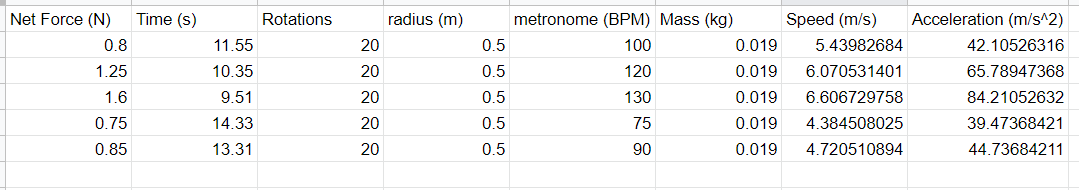
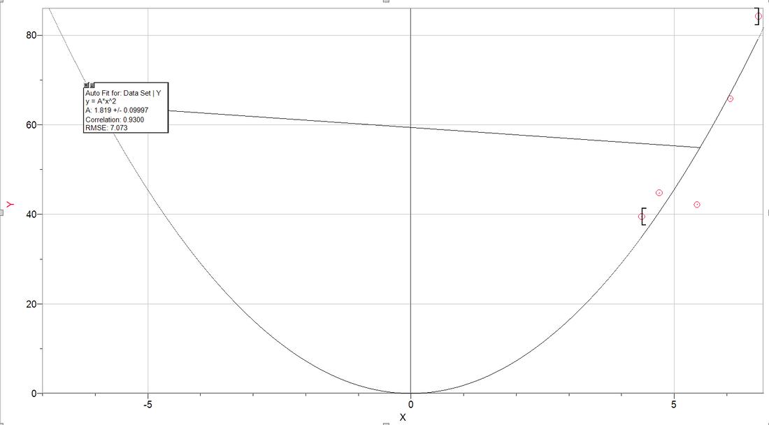
We had to make 2 main calculations to plug into the graph. We calculated the speed of the object by using rotations per second we calculated for the trial. We multiplied the Rotations/second by 2π0.5/1 revolution. 2πr represents the circumference of the circle the object is making in the air, in order to measure the distance traveled. 0.5 m is the radius of this circle. Once we found the total distance, we divided it by the elapsed time it took to revolve 20 times. This gave us the velocity of the object. To find the acceleration we used the equation F=ma. We divided the mass of the object (0.019 kg) from the tension force. That gives the accelerations for the specific data point. We plugged these values into the graph. We then fitted the graph to the model of A=cV^2 where c is a coefficient because it fits the model the best. The acceleration could never be negative because the force is always acting on the object. Similarly there cannot be an x intercept because the object is constantly changing direction.
Conclusion
We can conclude from this experiment that ultimately the relationship between centripetal acceleration and velocity is represented by the equation a = (v^2)/r . We were able to derive this equation from plugging in our variables to the model fit of the graph. We substituted 1/r as our c value, which is 1/0.5 which explains why our graph is so close to 2 for the coefficient. This equation a = (v^2)/r is significant because it allows us to find the acceleration and inversely the velocity of a centripetal object. Finally, this allows us to find the forces of centripetal velocity by using the speed acceleration, radius, and mass. This lab and the discovery of this equation is key to understanding centripetal motion.
Evaluating Procedures
We do not have a very high confidence level on this specific experiment due to the data collection. We only had 5 data points which made it hard to see a large trend. More importantly we had a small range with our largest value only being double the smallest value. This small range in data leads to a lot of uncertainty and lack of resembling fit. This can be improved by increasing the overall data points.
